SHRED Implementation#
This notebook walks the user through a standard SHRED implementation. After reading this notebook, you should be able to understand how to implement a SHRED model for you dataset.
The first step is to load your data. In this notebook, we will be using Sea-Surface Temperature data from NOAA. You can download the data from here. Place the SST_data.mat file in the top-level data/sst/ directory.
Imports and Parameters#
[8]:
%load_ext autoreload
%autoreload 2

import os
import pprint as pp
from typing import cast

import einops
import numpy as np
import torch

import shredx

smoke = os.environ.get("SMOKE", "False") == "True"  # Used for testing that the notebook runs

if smoke:
    input_length = 1
    n_epochs = 1
    lr = 1e-4
    forecast_length = 1
    n_sensors = 1
    device = "cpu"
else:
    input_length = 10
    n_epochs = 50
    lr = 1e-4
    forecast_length = 1
    n_sensors = 5
    device = "cuda" if torch.cuda.is_available() else "cpu"

np.random.seed(42)

%matplotlib inline
The autoreload extension is already loaded. To reload it, use:
  %reload_ext autoreload
Loading the Data#
The SST dataset can be loaded using our datasets module. The dataloader is a TimeSeriesDataset. This dataset allows for flexible input and output tensor configuration. It returns a tuple of two windows with input_length + forecast_length timesteps. You can have the input and output tensors be different, as long as they have the same number of timesteps. This allows you to train from sparse sensor measurements of a dense field and then output to POD modes (as in
SHRED-ROM) or to the full state field (as in base SHRED).
Here, we load the SST data so that the input and output tensors are the same.
[2]:
# Load dataset
train_ds, valid_ds, test_ds, metadata = shredx.datasets.datasets.load_sst_data(
    input_length=input_length, forecast_length=forecast_length
)

# Show values
sample = train_ds[0]
print("Input sample shape:", sample[0].shape)
print("Output sample shape:", sample[0].shape)  # Can output to POD modes instead if we want

n_timesteps = sample[0].shape[0]
n_rows = sample[0].shape[1]
n_cols = sample[0].shape[2]
n_channels = sample[0].shape[3]
Input sample shape: torch.Size([11, 180, 360, 1])
Output sample shape: torch.Size([11, 180, 360, 1])
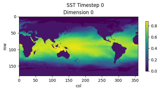
Data Visualization#
To visualize our data, we will be using the plots module. This allows us to plot our dense SST time series data.
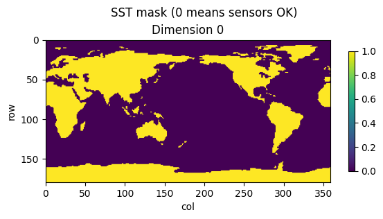
We also use the sst_zeros metadata to show where dynamics occur for this dataset.
[3]:
shredx.utils.plots.plot_timestep(sample[0][0], title="SST Timestep 0", save=False)

shredx.utils.plots.plot_timestep(metadata["sst_zeros"], title="SST mask (0 means sensors OK)", save=False)
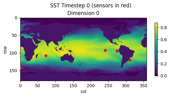
Sensor Extraction#
To extract sensors from our input sample, we use the sensors module and once again plot using the plots module.
[4]:
mask = metadata["sst_zeros"]
sensor_locations = shredx.utils.sensors.generate_static_sensors_from_mask(n_sensors, mask, dim_agnostic=True)
sensor_locations = cast(list[tuple[int, int]], sensor_locations)

print("Sensor locations:")
pp.pprint([{"x": x, "y": y} for x, y in sensor_locations])
print()

sensor_values = shredx.utils.sensors.extract_static_sensors(sample[0], sensor_locations)
print("Sensor values shape:", sensor_values.shape)
print()

shredx.utils.plots.plot_timestep(
    sample[0][0], title="SST Timestep 0 (sensors in red)", save=False, sensors=sensor_locations
)
Sensor locations:
[{'x': 143, 'y': 2},
 {'x': 95, 'y': 274},
 {'x': 121, 'y': 311},
 {'x': 108, 'y': 73},
 {'x': 93, 'y': 241}]

Sensor values shape: torch.Size([11, 5, 1])
Defining SHRED#
We will use the MixedModel class to define our SHRED model. We will use an LSTM as the encoder and an MLP as a decoder implemented in the LSTMEncoder and MLPDecoder classes. Here, we pass the sensor values into a newly initiated SHRED model. Note that the output to SHRED models are formatted as [batch, time, sequence_length, rows, columns, dimension]. In this case, time, sequence_length, and dimension are 1 and we reshape the output to [1, rows, columns].
The input to the encoder is of shape [batch, time, (sequence_length * dimension)] and the output of the decoder is of shape [batch, time, sequence_length, (rows * columns)].
[5]:
lstm_encoder = shredx.modules.rnn.LSTMEncoder(
    input_size=n_sensors * n_channels, hidden_size=n_sensors, num_layers=3, dropout=0.0, device=device
)
mlp_decoder = shredx.modules.mlp.MLPDecoder(
    in_dim=n_sensors, out_dim=n_rows * n_cols * n_channels, n_layers=2, dropout=0.0, device=device
)
shred = shredx.models.mixed_model.MixedModel(lstm_encoder, mlp_decoder)

# Squish sensor_values dimension and n_sensors to one dimension
sensor_values_batch = einops.rearrange(sensor_values, "t s 1 -> 1 t (s 1)")
if sensor_values_batch is None:
    raise ValueError("sensor_values_batch is None")
sensor_values_batch = sensor_values_batch.to(device)

# Verify we can pass data into SHRED
with torch.no_grad():
    output, _ = shred(sensor_values_batch)
    print("SHRED Output shape:", output.shape)
    output = einops.rearrange(output, "1 t s (r c) -> (1 t s) r c 1", r=n_rows, c=n_cols)
    print("SHRED Output reshaped:", output.shape)
None
SHRED Output shape: torch.Size([1, 1, 1, 64800])
SHRED Output reshaped: torch.Size([1, 180, 360, 1])
Training Loop#
We train SHRED to reconstruct the next timestep from the sparse sensor measurements.
[6]:
optimizer = torch.optim.Adam(shred.parameters(), lr=lr)
loss_fn = torch.nn.MSELoss()
losses = []

for i in range(n_epochs):
    for batch in train_ds:
        # Load data
        input_window, output_window = batch

        # Prepare inputs and outputs
        input_window = input_window[:input_length]
        output_window = output_window[input_length : input_length + forecast_length]
        input_window = input_window.to(device)
        output_window = output_window.to(device)

        # Prepare input sensors
        input_sensors = shredx.utils.sensors.extract_static_sensors(input_window, sensor_locations)
        input_sensors = einops.rearrange(input_sensors, "t s 1 -> 1 t (s 1)")
        input_sensors = input_sensors.to(device)

        # Pass into model
        optimizer.zero_grad()
        output, _ = shred(input_sensors)

        # Compute loss
        output = einops.rearrange(output, "1 t s (r c) -> (1 t s) r c 1", r=n_rows, c=n_cols)
        loss = loss_fn(output, output_window)
        loss.backward()
        optimizer.step()

        # Log loss
        losses.append(loss.item())

    # Print progress
    if i % 10 == 0 or i == n_epochs - 1:
        print(f"Epoch {i}, Loss: {loss.item()}")
Epoch 0, Loss: 0.002057179342955351
Epoch 10, Loss: 0.0009924274636432528
Epoch 20, Loss: 0.000846892362460494
Epoch 30, Loss: 0.0014453541953116655
Epoch 40, Loss: 0.0014395852340385318
Epoch 49, Loss: 0.00037358643021434546
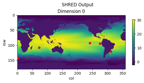
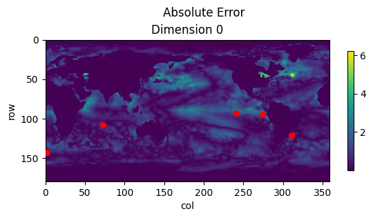
Visualizing Outputs#
Once SHRED is trained, we can pass in a set of test sensors and visualize the output. We use the metadata scalers to do the inverse min-max normalization of the output data.
[7]:
# Extract test sensors
sensor_values = shredx.utils.sensors.extract_static_sensors(test_ds[0][0], sensor_locations)
sensor_values_batch = einops.rearrange(sensor_values, "t s 1 -> 1 t (s 1)")
sensor_values_batch = sensor_values_batch.to(device)

# Verify we can pass data into SHRED
with torch.no_grad():
    output, _ = shred(sensor_values_batch)
    print("SHRED Output shape:", output.shape)
    output = einops.rearrange(output, "1 t s (r c) -> (1 t s) r c 1", r=n_rows, c=n_cols)
    print("SHRED Output reshaped:", output.shape)
    output = output[0].detach().cpu()

    # Inverse min-max scaling
    scaler = metadata["scalers"][0]
    output = shredx.utils.scaling.inverse_min_max_scale(output, original_min_max=scaler)
    expected = shredx.utils.scaling.inverse_min_max_scale(
        test_ds[0][1][input_length + forecast_length - 1], original_min_max=scaler
    )

    # Plot
    shredx.utils.plots.plot_timestep(expected, title="Expected Output", save=False, sensors=sensor_locations)
    shredx.utils.plots.plot_timestep(output, title="SHRED Output", save=False, sensors=sensor_locations)
    shredx.utils.plots.plot_timestep(
        torch.abs(output - expected), title="Absolute Error", save=False, sensors=sensor_locations
    )
SHRED Output shape: torch.Size([1, 1, 1, 64800])
SHRED Output reshaped: torch.Size([1, 180, 360, 1])